This work is supported by Anaconda Inc. and the Data Driven Discovery Initiative from the Moore Foundation.
Anaconda is interested in scaling the scientific python ecosystem. My current focus is on out-of-core, parallel, and distributed machine learning. This series of posts will introduce those concepts, explore what we have available today, and track the community’s efforts to push the boundaries.
You can download a Jupyter notebook demonstrating the analysis here.
Constraints
I am (or was, anyway) an economist, and economists like to think in terms of constraints. How are we constrained by scale? The two main ones I can think of are
- I’m constrained by size: My training dataset fits in RAM, but I have to predict for a much larger dataset. Or, my training dataset doesn’t even fit in RAM. I’d like to scale out by adopting algorithms that work in batches locally, or on a distributed cluster.
- I’m constrained by time: I’d like to fit more models (think hyper-parameter optimization or ensemble learning) on my dataset in a given amount of time. I’d like to scale out by fitting more models in parallel, either on my laptop by using more cores, or on a cluster.
These aren’t mutually exclusive or exhaustive, but they should serve as a nice framework for our discussion. I’ll be showing where the usual pandas + scikit-learn for in-memory analytics workflow breaks down, and offer some solutions for scaling out to larger problems.
This post will focus on cases where your training dataset fits in memory, but you must predict on a dataset that’s larger than memory. Later posts will explore into parallel, out-of-core, and distributed training of machine learning models.
Don’t forget your Statistics
Statistics is a thing1. Statisticians have thought a lot about things like sampling and the variance of estimators. So it’s worth stating up front that you may be able to just
SELECT *
FROM dataset
ORDER BY random()
LIMIT 10000;
and fit your model on a (representative) subset of your data. You may not need distributed machine learning. The tricky thing is selecting how large your sample should be. The “correct” value depends on the complexity of your learning task, the complexity of your model, and the nature of your data. The best you can do here is think carefully about your problem and to plot the learning curve.
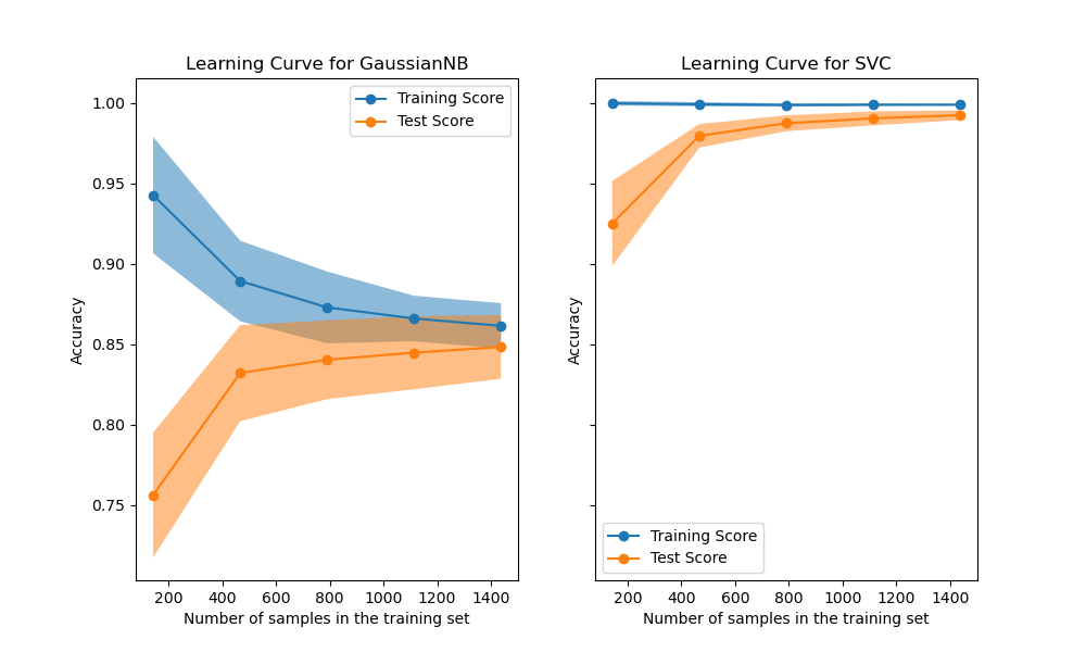
As usual, the scikit-learn developers do a great job explaining the concept in addition to providing a great library. I encourage you to follow that link. This gist is that—for some models on some datasets—training the model on more observations doesn’t improve performance. At some point the learning curve levels off and you’re just wasting time and money training on those extra observations.
For today, we’ll assume that we’re on the flat part of the learning curve. Later in the series we’ll explore cases where we run out of RAM before the learning curve levels off.
Fit, Predict
In my experience, the first place I bump into RAM constraints is when my training dataset fits in memory, but I have to make predictions for a dataset that’s orders of magnitude larger. In these cases, I fit my model like normal, and do my predictions out-of-core (without reading the full dataset into memory at once).
We’ll see that the training side is completely normal (since everything fits in RAM). We’ll see that dask let’s us write normal-looking pandas and NumPy code, so we don’t have to worry about writing the batching code ourself.
To make this concrete, we’ll use the (tried and true) New York City taxi dataset. The goal will be to predict if the passenger leaves a tip. We’ll train the model on a single month’s worth of data (which fits in my laptop’s RAM), and predict on the full dataset2.
Let’s load in the first month of data from disk:
dtype = {
    'vendor_name': 'category',
    'Payment_Type': 'category',
}

df = pd.read_csv("data/yellow_tripdata_2009-01.csv", dtype=dtype,
                 parse_dates=['Trip_Pickup_DateTime', 'Trip_Dropoff_DateTime'],)
df.head()
| vendor_name | Trip_Pickup_DateTime | Trip_Dropoff_DateTime | Passenger_Count | Trip_Distance | Start_Lon | Start_Lat | Rate_Code | store_and_forward | End_Lon | End_Lat | Payment_Type | Fare_Amt | surcharge | mta_tax | Tip_Amt | Tolls_Amt | Total_Amt | |
|---|---|---|---|---|---|---|---|---|---|---|---|---|---|---|---|---|---|---|
| 0 | VTS | 2009-01-04 02:52:00 | 2009-01-04 03:02:00 | 1 | 2.63 | -73.991957 | 40.721567 | NaN | NaN | -73.993803 | 40.695922 | CASH | 8.9 | 0.5 | NaN | 0.00 | 0.0 | 9.40 |
| 1 | VTS | 2009-01-04 03:31:00 | 2009-01-04 03:38:00 | 3 | 4.55 | -73.982102 | 40.736290 | NaN | NaN | -73.955850 | 40.768030 | Credit | 12.1 | 0.5 | NaN | 2.00 | 0.0 | 14.60 |
| 2 | VTS | 2009-01-03 15:43:00 | 2009-01-03 15:57:00 | 5 | 10.35 | -74.002587 | 40.739748 | NaN | NaN | -73.869983 | 40.770225 | Credit | 23.7 | 0.0 | NaN | 4.74 | 0.0 | 28.44 |
| 3 | DDS | 2009-01-01 20:52:58 | 2009-01-01 21:14:00 | 1 | 5.00 | -73.974267 | 40.790955 | NaN | NaN | -73.996558 | 40.731849 | CREDIT | 14.9 | 0.5 | NaN | 3.05 | 0.0 | 18.45 |
| 4 | DDS | 2009-01-24 16:18:23 | 2009-01-24 16:24:56 | 1 | 0.40 | -74.001580 | 40.719382 | NaN | NaN | -74.008378 | 40.720350 | CASH | 3.7 | 0.0 | NaN | 0.00 | 0.0 | 3.70 |
The January 2009 file has about 14M rows, and pandas takes about a minute to read the CSV into memory. We’ll do the usual train-test split:
X = df.drop("Tip_Amt", axis=1)
y = df['Tip_Amt'] > 0

X_train, X_test, y_train, y_test = train_test_split(X, y)

print("Train:", len(X_train))
print("Test: ", len(X_test))
Train: 10569309
Test:  3523104
Aside on Pipelines
The first time you’re introduced to scikit-learn, you’ll typically be shown how
you pass two NumPy arrays X and y straight into an estimator’s .fit
method.
from sklearn.linear_model import LinearRegression

est = LinearRegression()
est.fit(X, y)
Eventually, you might want to use some of scikit-learn’s pre-processing methods.
For example, we might impute missing values with the median and normalize the
data before handing it off to LinearRegression. You could do this “by hand”:
from sklearn.preprocessing import Imputer, StandardScaler

imputer = Imputer(strategy='median')
X_filled = imputer.fit_transform(X, y)

scaler = StandardScaler()
X_scaled = X_scaler.fit_transform(X_filled, y)

est = LinearRegression()
est.fit(X_scaled, y)
We set up each step, and manually pass the data through: X -> X_filled -> X_scaled.
The downside of this approach is that we now have to remember which
pre-processing steps we did, and in what order. The pipeline from raw data to
fit model is spread across multiple python objects. A better approach is to use
scikit-learn’s Pipeline object.
from sklearn.pipeline import make_pipeline

pipe = make_pipeline(
    Imputer(strategy='median'),
    StandardScaler(),
    LinearRegression()
)
pipe.fit(X, y)
Each step in the pipeline implements the fit, transform, and fit_transform
methods. Scikit-learn takes care of shepherding the data through the various
transforms, and finally to the estimator at the end. Pipelines have many
benefits but the main one for our purpose today is that it packages our entire
task into a single python object. Later on, our predict step will be a single
function call, which makes scaling out to the entire dataset extremely
convenient.
If you want more information on Pipelines, check out the scikit-learn
docs, this blog post, and my talk from
PyData Chicago 2016. We’ll be implementing some custom ones,
which is not the point of this post. Don’t get lost in the weeds here, I only
include this section for completeness.
Our Pipeline
This isn’t a perfectly clean dataset, which is nice because it gives us a chance to demonstrate some pandas’ pre-processing prowess, before we hand the data of to scikit-learn to fit the model.
from sklearn.pipeline import make_pipeline
# We'll use FunctionTransformer for simple transforms
from sklearn.preprocessing import FunctionTransformer
# TransformerMixin gives us fit_transform for free
from sklearn.base import TransformerMixin
There are some minor differences in the spelling on “Payment Type”:
df.Payment_Type.cat.categories
Index(['CASH', 'CREDIT', 'Cash', 'Credit', 'Dispute', 'No Charge'], dtype='object')
We’ll reconcile that by lower-casing everything with a .str.lower(). But
resist the temptation to just do that imperatively inplace! We’ll package it up
into a function that will later be wrapped up in a FunctionTransformer.
def payment_lowerer(X):
    return X.assign(Payment_Type=X.Payment_Type.str.lower())
I should note here that I’m using
.assign
to update the variables since it implicitly copies the data. We don’t want to
be modifying the caller’s data without their consent.
Not all the columns look useful. We could have easily solved this by only reading in the data that we’re actually going to use, but let’s solve it now with another simple transformer:
class ColumnSelector(TransformerMixin):
    "Select `columns` from `X`"
    def __init__(self, columns):
        self.columns = columns

    def fit(self, X, y=None):
        return self

    def transform(self, X, y=None):
        return X[self.columns]
Internally, pandas stores datetimes like Trip_Pickup_DateTime as a 64-bit
integer representing the nanoseconds since some time in the 1600s. If we left
this untransformed, scikit-learn would happily transform that column to its
integer representation, which may not be the most meaningful item to stick in
a linear model for predicting tips. A better feature might the hour of the day:
class HourExtractor(TransformerMixin):
    "Transform each datetime in `columns` to integer hour of the day"
    def __init__(self, columns):
        self.columns = columns

    def fit(self, X, y=None):
        return self

    def transform(self, X, y=None):
        return X.assign(**{col: lambda x: x[col].dt.hour
                           for col in self.columns})
Likewise, we’ll need to ensure the categorical variables (in a statistical
sense) are categorical dtype (in a pandas sense). We want categoricals so that
we can call get_dummies later on without worrying about missing or extra
categories in a subset of the data throwing off our linear algebra (See my
talk for more details).
class CategoricalEncoder(TransformerMixin):
    """
    Convert to Categorical with specific `categories`.

    Examples
    --------
    >>> CategoricalEncoder({"A": ['a', 'b', 'c']}).fit_transform(
    ...     pd.DataFrame({"A": ['a', 'b', 'a', 'a']})
    ... )['A']
    0    a
    1    b
    2    a
    3    a
    Name: A, dtype: category
    Categories (2, object): [a, b, c]
    """
    def __init__(self, categories):
        self.categories = categories

    def fit(self, X, y=None):
        return self

    def transform(self, X, y=None):
        X = X.copy()
        for col, categories in self.categories.items():
            X[col] = X[col].astype('category').cat.set_categories(categories)
        return X
Finally, we’d like to normalize the quantitative subset of the data. Scikit-learn has a StandardScaler, which we’ll mimic here, to just operate on a subset of the columns.
class StandardScaler(TransformerMixin):
    "Scale a subset of the columns in a DataFrame"
    def __init__(self, columns):
        self.columns = columns

    def fit(self, X, y=None):
        # Yes, non-ASCII symbols can be a valid identfiers in python 3
        self.μs = X[self.columns].mean()
        self.σs = X[self.columns].std()
        return self

    def transform(self, X, y=None):
        X = X.copy()
        X[self.columns] = X[self.columns].sub(self.μs).div(self.σs)
        return X
Side-note: I’d like to repeat my desire for a library of Transformers that
work well on NumPy arrays, dask arrays, pandas DataFrames and dask dataframes.
I think that’d be a popular library. Essentially everything we’ve written could
go in there and be imported.
Now we can build up the pipeline:
# The columns at the start of the pipeline
columns = ['vendor_name', 'Trip_Pickup_DateTime',
           'Passenger_Count', 'Trip_Distance',
           'Payment_Type', 'Fare_Amt', 'surcharge']

# The mapping of {column: set of categories}
categories = {
    'vendor_name': ['CMT', 'DDS', 'VTS'],
    'Payment_Type': ['cash', 'credit', 'dispute', 'no charge'],
}

scale = ['Trip_Distance', 'Fare_Amt', 'surcharge']

pipe = make_pipeline(
    ColumnSelector(columns),
    HourExtractor(['Trip_Pickup_DateTime']),
    FunctionTransformer(payment_lowerer, validate=False),
    CategoricalEncoder(categories),
    FunctionTransformer(pd.get_dummies, validate=False),
    StandardScaler(scale),
    LogisticRegression(),
)
pipe
[('columnselector', <__main__.ColumnSelector at 0x1a2c726d8>),
 ('hourextractor', <__main__.HourExtractor at 0x10dc72a90>),
 ('functiontransformer-1', FunctionTransformer(accept_sparse=False,
           func=<function payment_lowerer at 0x17e0d5510>, inv_kw_args=None,
           inverse_func=None, kw_args=None, pass_y='deprecated',
           validate=False)),
 ('categoricalencoder', <__main__.CategoricalEncoder at 0x11dd72f98>),
 ('functiontransformer-2', FunctionTransformer(accept_sparse=False,
           func=<function get_dummies at 0x10f43b0d0>, inv_kw_args=None,
           inverse_func=None, kw_args=None, pass_y='deprecated',
           validate=False)),
 ('standardscaler', <__main__.StandardScaler at 0x162580a90>),
 ('logisticregression',
  LogisticRegression(C=1.0, class_weight=None, dual=False, fit_intercept=True,
           intercept_scaling=1, max_iter=100, multi_class='ovr', n_jobs=1,
           penalty='l2', random_state=None, solver='liblinear', tol=0.0001,
           verbose=0, warm_start=False))]
We can fit the pipeline as normal:
%time pipe.fit(X_train, y_train)
This take about a minute on my laptop. We can check the accuracy (but again, this isn’t the point)
>>> pipe.score(X_train, y_train)
0.9931

>>> pipe.score(X_test, y_test)
0.9931
It turns out people essentially tip if and only if they’re paying with a card, so this isn’t a particularly difficult task. Or perhaps more accurately, tips are only recorded when someone pays with a card.
Scaling Out with Dask
OK, so we’ve fit our model and it’s been basically normal. Maybe we’ve been overly-dogmatic about doing everything in a pipeline, but that’s just good model hygiene anyway.
Now, to scale out to the rest of the dataset. We’ll predict the probability of tipping for every cab ride in the dataset (bearing in mind that the full dataset doesn’t fit in my laptop’s RAM, so we’ll do it out-of-core).
To make things a bit easier we’ll use dask, though it isn’t strictly necessary for this section. It saves us from writing a for loop (big whoop). Later on well see that we can, reuse this code when we go to scale out to a cluster (that part is pretty cool, actually). Dask can scale down to a single laptop, and up to thousands of cores.
import dask.dataframe as dd

df = dd.read_csv("data/*.csv", dtype=dtype,
                 parse_dates=['Trip_Pickup_DateTime', 'Trip_Dropoff_DateTime'],)

X = df.drop("Tip_Amt", axis=1)
X is a dask.dataframe, which can be mostly be treated like a pandas
dataframe (internally, operations are done on many smaller dataframes). X has
about 170M rows (compared with the 14M for the training dataset).
Since scikit-learn isn’t dask-aware, we can’t simply call
pipe.predict_proba(X). At some point, our dask.dataframe would be cast to a
numpy.ndarray, and our memory would blow up. Fortunately, dask has some nice
little escape hatches for dealing with functions that know how to operate on
NumPy arrays, but not dask objects. In this case, we’ll use map_partitions.
yhat = X.map_partitions(lambda x: pd.Series(pipe.predict_proba(x)[:, 1],
                                            name='yhat'),
                        meta=('yhat', 'f8'))
map_partitions will go through each partition in your dataframe (one per
file), calling the function on each partition. Dask worries about stitching
together the result (though we provide a hint with the meta keyword, to say
that it’s a Series with name yhat and dtype f8).
Now we can write it out to disk (using parquet rather than CSV, because CSVs are evil).
yhat.to_frame().to_parquet("data/predictions.parq")
This takes about 9 minutes to finish on my laptop.
Scaling Out (even further)
If 9 minutes is too long, and you happen to have a cluster sitting around, you can repurpose that dask code to run on the distributed scheduler. I’ll use dask-kubernetes, to start up a cluster on Google Cloud Platform, but you could also use dask-ec2 for AWS, or dask-drmaa or dask-yarn if already have access to a cluster from your business or institution.
dask-kubernetes create scalable-ml
This sets up a cluster with 8 workers and 54 GB of memory.
The next part of this post is a bit fuzzy, since your teams will probably have different procedures and infrastructure around persisting models. At my old job, I wrote a small utility for serializing a scikit-learn model along with some metadata about what it was trained on, before dumping it in S3. If you want to be fancy, you should watch this talk by Rob Story on how Stripe handles these things (it’s a bit more sophisticated than my “dump it on S3” script).
For this blog post, “shipping it to prod” consists of a joblib.dump(pipe, "taxi-model.pkl") on our laptop, and copying it to somewhere the cluster can
load the file. Then on the cluster, we’ll load it up, and create a Client to
communicate with our cluster’s workers.
from distributed import Client
from sklearn.externals import joblib

pipe = joblib.load("taxi-model.pkl")
c = Client('dask-scheduler:8786')
Depending on how your cluster is set up, specifically with respect to having a shared-file-system or not, the rest of the code is more-or-less identical. If we’re using S3 or Google Cloud Storage as our shared file system, we’d modify the loading code to read from S3 or GCS, rather than our local hard drive:
df = dd.read_csv("s3://bucket/yellow_tripdata_2009*.csv",
                 dtype=dtype,
                 parse_dates=['Trip_Pickup_DateTime', 'Trip_Dropoff_DateTime'],
                 storage_options={'anon': True})
df = c.persist(df)  # persist the dataset in distributed memory
                    # across all the workers in the Dataset
X = df.drop("Tip_Amt", axis=1)
y = df['Tip_Amt'] > 0
Computing the predictions is identical to our out-of-core-on-my-laptop code:
yhat = X.map_partitions(lambda x: pd.Series(pipe.predict_proba(x)[:, 1], name='yhat'),
                        meta=('yhat', 'f8'))
And saving the data (say to S3) might look like
yhat.to_parquet("s3://bucket/predictions.parq")
The loading took about 4 minutes on the cluster, the predict about 10 seconds, and the writing about 1 minute. Not bad overall.
Wrapup
Today, we went into detail on what’s potentially the first scaling problem you’ll hit with scikit-learn: you can train your dataset in-memory (on a laptop, or a large workstation), but you have to predict on a much larger dataset.
We saw that the existing tools handle this case quite well. For training, we
followed best-practices and did everything inside a Pipeline object. For
predicting, we used dask to write regular pandas code that worked out-of-core
on my laptop or on a distributed cluster.
If this topic interests you, you should watch this talk by Stephen Hoover on how Civis is scaling scikit-learn.
In future posts we’ll dig into
- how dask can speed up your existing pipelines by executing them in parallel
- scikit-learn’s out of core API for when your training dataset doesn’t fit in memory
- using dask to implement distributed machine learning algorithms
Until then I would really appreciate your feedback. My personal experience using scikit-learn and pandas can’t cover the diversity of use-cases they’re being thrown into. You can reach me on Twitter @TomAugspurger or by email at mailto:tom.w.augspurger@gmail.com. Thanks for reading!